线性回归——梯度下降法求解

• LMS algorithm
• Batch Gradient Descent
• Repeat until convergence {
• Stochastic Gradient Descent

LMS algorithm

We want to choose $\theta$ so as to minimize $J(\theta ).$ To do so, let's use a search algorithm that starts with some “initial guess” for $\theta$, and that repeatedly changes $\theta$ to make $J(\theta )$ smaller, until hopefully we converge to a value of $\theta$ that minimizes $J(\theta ).$ Specifically, let's consider the gradient descent algorithm, which starts with some initial $\theta$, and repeatedly performs the update:

$${\theta }_j:={\theta }_j-\alpha \frac{\partial }{\partial {\theta }_j}J(\theta ).$$

(This update is simultaneously performed for all values of $j=0,\dots ,d.)$ Here, $\alpha$ is called the learning rate. This is a very natural algorithm that repeatedly takes a step in the direction of steepest decrease of $J.$

In order to implement this algorithm, we have to work out what is the partial derivative term on the right hand side. Let's first work it out for the case of if we have only one training example $(x,y)$, so that we can neglect the sum in the definition of $J$. We have:

$$\begin{array}{rl}\frac{\partial }{\partial {\theta }_j}J(\theta )& =\frac{\partial }{\partial {\theta }_j}\frac{1}{2}{\left(h_{\theta }(x)-y\right)}^2\\ & =2\cdot \frac{1}{2}\left(h_{\theta }(x)-y\right)\cdot \frac{\partial }{\partial {\theta }_j}(h_{\theta }(x)-y)\\ & =(h_{\theta }(x)-y)\cdot \frac{\partial }{\partial {\theta }_j}\left(\sum _{i=0}^d{\theta }_i{x}_i-y\right)\\ & =\left(h_{\theta }(x)-y\right)x_j\end{array}$$ For a single training example, this gives the update rule:${}^1$

$${\theta }_j:={\theta }_j+\alpha \left(y^{(i)}-h_{\theta }(x^{(i)})\right)x_j^{(i)}.$$

The rule is called the LMS update rule (LMS stands for “least mean squares”), and is also known as the Widrow-Hoff learning rule. This rule has several properties that seem natural and intuitive. For instance, the magnitude of the update is proportional to the error term $(y^{(i)}-h_{\theta }(x^{(i)}));$ thus, for instance, if we are encountering a training example on which our prediction nearly matches the actual value of $y^{(i)}$, then we find that there is little need to change the parameters; in contrast, a larger change to the parameters will be made if our prediction $h_{\theta }(x^{(i)})$ has a large error (i.e., if it is very far from $y^{(i)}).$

We'd derived the LMS rule for when there was only a single training example. There are two ways to modify this method for a training set of more than one example.

Batch Gradient Descent

The first is replace it with the following algorithm:

Repeat until convergence $\{$

$${\theta }_j:={\theta }_j+\alpha \sum _{i=1}^n\left(y^{(i)}-h_{\theta }(x^{(i)})\right)x_j^{(i)},\text{(for every }j)$$

}

By grouping the updates of the coordinates into an update of the vector $\theta$, we can rewrite update (1.1) in a slightly more succinct way:

$$\theta :=\theta +\alpha \sum _{i=1}^n\left(y^{(i)}-h_{\theta }(x^{(i)})\right)x^{(i)}$$

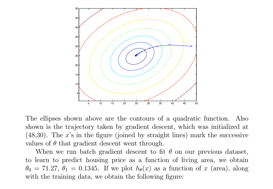
The reader can easily verify that the quantity in the summation in the update rule above is just $\partial (J(\theta ))/\partial {\theta }_j$( for the original definition of $J$) . So, this is simply gradient descent on the original cost function $J.$ This method looks at every example in the entire training set on every step, and is called batch gradient descent. Note that, while gradient descent can be susceptible to local minima in general, the optimization problem we have posed here for linear regression has only one global, and no other local, optima; thus gradient descent always converges (assuming the learning rate $\alpha$ is not too large) to the global minimum. Indeed, $J$ is a convex quadratic function. Here is an example of gradient descent as it is run to minimize a quadratic function.

Stochastic Gradient Descent

The above results were obtained with batch gradient descent. There is an alternative to batch gradient descent that also works very well. Consider the following algorithm:

Loop $\{$ for $i=1$ to $n,$

$${\theta }_j:={\theta }_j+\alpha \left(y^{(i)}-h_{\theta }(x^{(i)})\right)x_j^{(i)},\text{(for every }j)$$

$\}$

By grouping the updates of the coordinates into an update of the vector $\theta$, we can rewrite update (1.2) in a slightly more succinct way:

$$\theta :=\theta +\alpha \left(y^{(i)}-h_{\theta }(x^{(i)})\right)x^{(i)}$$

In this algorithm, we repeatedly run through the training set, and each time we encounter a training example, we update the parameters according to the gradient of the error with respect to that single training example only. This algorithm is called stochastic gradient descent (also incremental gradient descent). Whereas batch gradient descent has to scan through the entire training set before taking a single step—a costly operation if $n$ is large—stochastic gradient descent can start making progress right away, and continues to make progress with each example it looks at. Often, stochastic gradient descent gets θ “close” to the minimum much faster than batch gradient descent. (Note however that it may never “converge” to the minimum, and the parameters θ will keep oscillating around the minimum of J(θ); but in practice most of the values near the minimum will be reasonably good approximations to the true minimum.)

For these reasons, particularly when the training set is large, stochastic gradient descent is often preferred over batch gradient descent.