线性回归

• 概述
• 小结

概述

Given data like this, how can we learn to predict the prices of other houses in Portland, as a function of the size of their living areas?

To establish notation for future use, we'll use $x^{(i)}$ to denotc the “input” variables (living area in this example), also called input featurcs, and $y^{(i)}$ to denote the “output” or target variable that we are trying to predict $(\mathrm{price}).$ A pair $(x^{(i)},y^{(i)})$ is called a training example, and the dataset that we'll be using to learn—a list of $n$ training examples $\{(x^{(i)},y^{(i)});i=$ $1,\dots ,n\}$—is called a training set. Note that the superscript “$(i)$” in the notation is simply an index into the training set, and has nothing to do with exponentiation. We will also use $\chi$ denote the space of input values, and $\gamma$ the space of output values. In this example, $\mathcal{X}=\mathcal{Y}=\mathbb{R}.$

To describe the supervised learning problem slightly more formally, our goal is, given a training set, to learn a function $h:\mathcal{X}\mapsto \mathcal{Y}$ so that $h(x)$ is a “good” predictor for the corresponding value of $y.$ For historical reasons, this function h is called a hypothesis.

When the target variable that we're trying to predict is continuous, such as in our housing example, we call the learning problem a regression problem.When $y$ can take on only a small number of discrete values (such as if, given the living area, we wanted to predict if a dwelling is a house or an apartment, say), we call it a classification problem.

Here, the $x$'s are two-dimensional vectors in ${\mathbb{R}}^2$. For instance, $x_1^{(i)}$ is the living area of the $i$-th house in the training set, and $x_2^{(i)}$ is its number of bedrooms. (In general, when designing a learning problem, it will be up to you to decide what features to choose, so if you are out in Portland gathering housing data, you might also decide to include other features such as whether each house has a fireplace, the number of bathrooms, and so on. We'll say more about feature selection later, but for now let's take the features as given.)

To perform supervised learning, we must decide how we're going to represent functions/hypotheses $h$ in a computer. As an initial choice, let's say we decide to approximate $y$ as a linear function of $x:$

$$\begin{array}{r}{h}_{\theta }(x)={\theta }_0+{\theta }_1{x}_1+{\theta }_2{x}_2\end{array}$$

Here, the ${\theta }_i$ 's are the parameters (also called weights) parameterizing the space of linear functions mapping from $\chi$ to $\gamma$. When there is no risk of confusion, we will drop the $\theta$ subscript in $h_{\theta }(x)$, and write it more simply as $h(x).$ To simplify our notation, we also introduce the convention of letting $x_0=1$(this is the intercept term), so that

$$h(x)=\sum _{i=0}^d{\theta }_i{x}_i={\theta }^{T}x,$$

where on the right-hand side above we are viewing $\theta$ and $x$ both as vectors, and here $d$ is the number of input variables (not counting $x_0).$

Now, given a training set, how do we pick, or learn, the parameters $\theta ?$ One reasonable method seems to be to make $h(x)$ close to $y$, at least for the training examples we have. To formalize this, we will define a function that measures, for each value of the $\theta$'s, how close the $h(x^{(i)})$'s are to the corresponding $y^{(i),}$s. We define the $\cos$t function:

$$\begin{array}{rl}J(\theta )& =\frac{1}{2}\sum _{i=1}^n(h_{\theta }(x^{(i)})-y^{(i)}{)}^2.\end{array}$$

If you've seen linear regression before, you may recognize this as the familian least-squares cost function that gives rise to the ordinary least squares regression model. Whether or not you have seen it previously, let's keep going, and we'll eventually show this to be a special case of a much broader family of algorithms.

两种求解方式的比较：

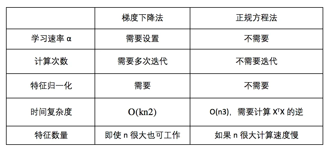
可见特征方程得到的是解析解，无需迭代，也没有设置学习速率的繁琐，需要特征归一化，但是求解正规方程需要求矩阵的逆，然而不是所有的矩阵都可逆，而且有些可逆矩阵的求逆极其耗费时间，所以特征方程法看似简单，其实使用场景并不多。只有当特征值比较小的时候，可以考虑使用特征方程法。

小结

线性回归模型是最简单的模型，但是麻雀虽小，五脏俱全，在这里，我们利用最小二乘误差得到了闭式解。同时也发现，在噪声为高斯分布的时候，MLE 的解等价于最小二乘误差，而增加了正则项后，最小二乘误差加上 L2 正则项等价于高斯噪声先验下的 MAP解，加上 L1 正则项后，等价于 Laplace 噪声先验。

传统的机器学习方法或多或少都有线性回归模型的影子：

1. 线性模型往往不能很好地拟合数据，因此有三种方案克服这一劣势：
   1. 对特征的维数进行变换，例如多项式回归模型就是在线性特征的基础上加入高次项。
   2. 在线性方程后面加入一个非线性变换，即引入一个非线性的激活函数，典型的有线性分类模型如感知机。
   3. 对于一致的线性系数，我们进行多次变换，这样同一个特征不仅仅被单个系数影响，例如多层感知机（深度前馈网络）。
2. 线性回归在整个样本空间都是线性的，我们修改这个限制，在不同区域引入不同的线性或非线性，例如线性样条回归和决策树模型。
3. 线性回归中使用了所有的样本，但是对数据预先进行加工学习的效果可能更好（所谓的维数灾难，高维度数据更难学习），例如 PCA 算法和流形学习。